
Solving Linear Programming Using the Graphical Method
What is Linear Programming?
Linear programming is a mathematical technique used to determine the best possible outcome from a mathematical model, in which the requirements and objective have linear relationships. It consists of an objective function that needs to be optimized with a set of constraints that will define the feasible region.
Linear programming is known to be used in various fields such as, finance, manufacturing, logistics, business, and many more. It is mainly used to maximize profit, minimize cost, optimize distribution, and efficient investment allocations.
The graphical method is one way to solve a linear programming problem. However, it is applicable when there are only two decision variables. Meanwhile, for larger problems, computational methods such as the simplex method will be a more suitable choice.
Elements of Linear Programming
- Problem and Goal: This element identifies what needs to be solved or the goal to be achieved (e.g., optimization, maximization, minimization).
- Decision Variables: It represents the quantities that will be determined (e.g., number of products to be produced).
- Objective Function: It is a mathematical expression that needs to be maximized or minimized (e.g., max. profit = 3x + 2y).
- Constraints: It is the restrictions or limitations on the resources (e.g., material availability, labor hours).
- Feasible Region: It is the area on the graph where all the constraints overlap, representing possible solutions.
- Corner points: These are the points where the constraints intersect, which will then be evaluated to find out the optimal solution.
Steps to Solve a Linear Programming Problem Using the Graphical Method
- Define the problem and goal
Find out the problem that needs to be solved or the goal wished to be achieved.
- Identify the decision variables
Determine the key variables that can affect the outcome. These variables are what will be adjusted to optimize the objective function.
- Define the objective function
The objective function is the formula that needs to be maximized or minimized. It is typically a linear equation that will represent profit, cost, or other measurable outcomes.
- Establish the constraints
Constraints are the limitations or restrictions in the problem, such as available resources, budget limits, production capacity, or labor hours. It is usually written as linear inequalities that needs to be satisfied.
- Plot the constraints on a graph
Convert the constraint inequalities into equations and graph out the boundary lines on a coordinate plane, where the x- and y-axis represent the decision variables. One way to find two points for each line is to set x = 0 and solve for y, and vice versa.
- Determine the feasible region
Shade the feasible side of each constraint (the region where all constraints hold true). The feasible region is the area on the graph where all constraints overlap. This region represents all possible solutions that satisfy the constraints.
- Identify the corner points
The corner points, also known as vertices, are the points where the boundary lines intersect within the feasible region. Methods such as substitution and elimination can also be used to identify the points.
- Evaluate the objective function at each corner point
For each corner points coordinates, substitute the x and y value into the objective function. Compare the results of the objective function from each corner point to determine the maximum or minimum value.
- Interpret the solution
The corner point that gives the best value, usually either maximum or minimum (based on the problem or goal), is the optimal solution. Hence, that will be the best decision for the given problem.
Example Question
A factory produces two types of products: Product A and Product B. The company wants to determine the number of each product to produce in order to maximize profit while considering resource limitations.
Given information:
- Each unit of Product A gives a profit of $5.
- Each unit of Product B gives a profit of $3.
- Each unit of Product A requires 2 hours of production, while each unit of Product B requires only 1 hour.
- The factory has a total of 10 machine hours available.
- Each unit of Product A requires 1 hour of labor, while each unit of Product B needs 2 hours.
- The factory has a total of 8 labor hours available.
Solution
Problem: Optimizing profit
Goal: Maximizing profit
Let:
- x = number of product A produced
- y = number of product B produced
- Z = profit
Decision variables: x and y
Objective Function: max Z = 5x + 3y
Constraints:
- Machine hours: 2x + y ≤ 10
- Labor hours: x + 2y ≤ 8
- x ≥ 0
- y ≥ 0
Equations for graphical method:
- x ≥ 0
- y ≥ 0
For 2x + y ≤ 10,
- x ≤ 5, coordinate: (5, 0)
- y ≤ 10, coordinate: (0, 10)
For x + 2y ≤ 8,
- x ≤ 8, coordinate (8,0)
- y ≤ 4, coordinate: (0, 4)
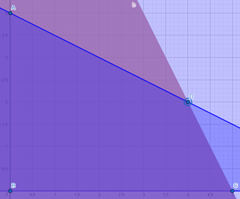
Corner points:
- (0,0)
- (0,4)
- (4,2)
- (5,0)
Substitute x and y values from the corner points into the objective function:
Objective function: Z = 5x + 3y
At (0,0):
Z = 5(0) + 3(0) = 0
At (0,4):
Z = 5(0) + 3(4) = 12
At (4,2):
Z = 5(4) + 3(2) = 26
At (5,0):
Z = 5(5) + 3(0) = 25
Optimal Solution
The highest profit is 26, achieved at corner point (4,2). This means that the company should produce 4 units of Product A and 2 units of Product B to maximize profit, which is when they gained the highest profit of 26.

Comments :